Map of the world’s languages

Esperanto  Dansk

Plots

Thanks to the AJSP database by the Max Planck institute, I was able to follow the method of Müller and group and make these plots using MDS(see Methods).

Discussion

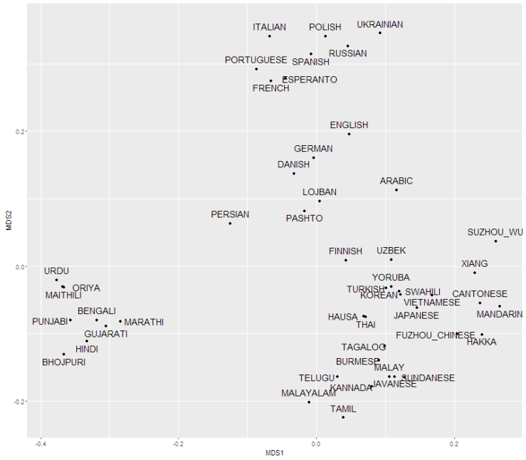
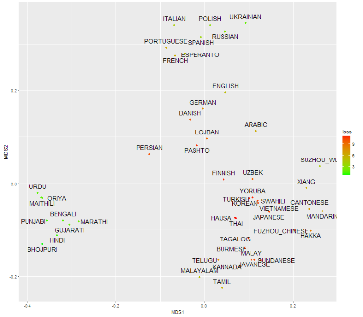
There are generally big differences between languages with the chosen distance measure. Even though the distance matrix has some obvious language groups, the languages are mostly distant. In addition, the MDS plot has many points which do not fit well to their assigned position. There are simply not enough space to distribute the languages without putting them too close or too distant from each other. Languages need a higher dimensional space to be portrayed better.

Esperanto vs Lojban

It is easiest to learn languages close to one’s native language(Isphording, I.E. and Otten, S., 2011), which is lucky for us europeans, because we learn English relatively easy. Esperanto, which I wrote fondly of in my previous post, is an easy language which is made to give more people easy access to a common language. Esperanto is often accused of being European. People say that as a candidate to a global second language, it should not belong to a specific language group. Esperanto is obviously a european language, but what is the alternative? When languages reside in such a high-dimensional space, a fusion of all languages would also be far away from all languages. It is illustrated by Lojban which was calculated in 1987 based on the 6 languages mandarin, english, spanish, hindi, arabic and russian. Lojban does get positioned in the middle of the MDS plot and is also just classified into the european language group by the phylogeny. Yet, the distances between Lojban and all other languages are large. Lojban is only in the middle of the MDS plot because no language wants it close. So measured with this language measure Lojban is as difficult to learn for everybody as esperanto is for non-europeans.

Methods

The Swadesh list is a list of the 100 most human concepts like I, who, mountain, hear, big and so on. Translations of the words in different languages are used to measure distance between those languages. After its creation the list was first extended to 207 words to increase the statistical power, but then it was reduced to the 40 words which carry most of the statistical power. (It seems that one should use a better statistical model instead, but I also think that about many things).

The Max Planck institute made the database AJSP containing the Swadesh list for more than 7000 languages. All translations are written in the same phonetic alphabet, which makes systematic approaches possible. Müller and coworkers did the following:

• The distance between two words is the normalized Levenshtein distance(LDND).
  • The Levenshtein distance(LD) is the smallest number of operations that it takes to transform one word into the other.
    • An operation is either a substitution, removal or addition of one letter.
  • The normalization consists of two steps.
    • Dividing the distance, LD, with the length of the longest word. The result is LDN
    • Dividing LDN with the average LDN of other words from those two languages
• The distance between two languages is the average distance between the Swadesh list words for the two languages.
• Pairwise distances between all languages make a phylogeny over all languages using the method Neighbour joining.
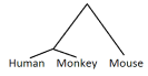
  • A phylogeny explains the evolutionary history between elements as is done for Human, monkey and mouse here: 

I mostly recreate the procedure of the Müller group, but I make some other choices to obtain a ‘map’ of the languages

• The distance between two words is the normalized Levenshtein distance(LDND LDN).
  • The Levenshtein distance(LD) is the smallest number of operations that it takes to transform one word into the other.
    • An operation is either a substitution, removal or addition of one letter.
  • The normalization consists of two one steps.
    • Dividing the distance, LD, with the length of the longest word. The result is LDN
    • Dividing LDN with the average LDN of other words from those two languages
• The distance between two languages is the average distance between the Swadesh list words for the two languages.
• Pairwise distances between all some languages make a phylogeny over all some languages using the method Neighbour joining.
  • A phylogeny explains the evolutionary history between elements as is done for Human, monkey and mouse here: 

• Pairwise distances between some languages make a ‘map’ of those languages using Multidimensional scaling(MDS).
  • Multidiemnsional scaling transforms a collection of pairwise distances to points in an n-dimensional plane. Imagine that we knew all pairwise distances between cities in Denmark and not the actual positions of the cities. Then MDS(with n=2) would produce a good estimate of how the map of danish cities would look like. MDS achieves this by minimizing the differences between the actual distances and the distances on the estimated map.
• I plot the distance matrix
  • In the distance matrix each row and each column correspond to a language. An entry is the distance between the row language and column language.

I did not use LDND because I think it is strange and not really necessary. I only used a subset of the languages because I wanted to make a small plot. I included the 45 languages with the highest numbers of native speakers, and my love/love-to-hate languages danish, Esperanto, Lojban and finnish. In the MDS calculations these 4 languages were weighed almost 0 in order not to let the plot be influenced by my hobbies.

The data set can be downloaded from the AJSP webpage(to do exactly like me, you should download the .zip-file Dataset in CLDF [10.9MB]). My source code is on github in the new fancy Rstudio Notebook format.